| (all) |
[R] arch, p. 76, Syntax
In the syntax diagram, an asterisk is required with the use of a "stub" in
the score() option.
|
... score(newvarlist | stub) ... |
... score(newvarlist | stub*) ... |
|
|
(all) |
[R] arch, p.
81, Syntax for predict
Add yresiduals to the available statistics list for
predict. Insert the following statement.
|
yresiduals residuals or predicted innovations
in y—the undifferenced series |
|
|
(all) |
[R] arch, p. 81, Options, saarch(numlist) option,
second paragraph
|
saarch() may not ... with tarch(), narch(), ...
|
saarch() may not ... with narch(), ... |
|
|
(all) |
[R] arch, p. 89, Options for predict.
Add the following paragraph describing the yresiduals option.
|
yresiduals calculates the residuals in terms of depvar,
even if the model was specified in terms of, say, D.depvar.
As with residuals, the yresiduals are computed from
the model including any ARMA component. If option
structural is specified, any ARMA component is ignored and
yresiduals are the residuals from the structural equation;
see structural below.
|
|
|
(all) |
[R] arima, p. 111, Syntax, Full syntax
In the syntax diagram an asterisk is required with the use of a “stub”
in the score() option.
|
... score(newvarlist | stub) ... |
... score(newvarlist | stub*) ... |
|
|
(all) |
[R] arima, p. 111, Syntax for predict
Add yresiduals to the available statistics list for
predict. Insert the following statement.
|
yresiduals residuals or predicted innovations
in y—the undifferenced series
|
|
|
(all) |
[R] arima, p. 116, Options for predict
Add the following paragraph describing the yresiduals option.
|
yresiduals calculates the residuals in terms of depvar,
even if the model was specified in terms of, say, D.depvar.
As with residuals, the yresiduals are computed from
the model including any ARMA component. If option
structural is specified, any ARMA component is ignored and
yresiduals are the residuals from the structural equation;
see structural below.
|
|
|
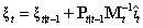
(1,2) |
[R] arima, p. 125, Methods and Formulas, eq. (12)
|
|
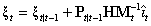
(1,2) |
[R] arima, p. 125, Methods and Formulas, eq. (13)
|
|
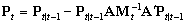
(3) |
[R] arima, p. 125, Methods and Formulas, eq. (13)
|
|
(all) |
[R] biprobit, p. 132, Syntax
A comma is missing in the description of the syntax for equation1 and
equation2.
|
... [ varlist ] [ offset(varname) ...
|
... [ varlist ] [, offset(varname) ...
|
|
|
(all) |
[R] biprobit, p. 133, Description
| biprobit estimates maximum-likelihood probit models
with sample selection. |
biprobit estimates maximum-likelihood two-equation
probit models—either a bivariate probit or a seemingly
unrelated probit (limited to two equations). |
|
|
(all) |
[R] ci, p. 194, Syntax
|
ci varlist [weight] ... |
ci [varlist] [weight] ... |
|
|
(all) |
[R] confirm, p. 243, Syntax
Keyword new cannot be abbreviated.
confirm [new] file
filename
confirm [new | ... ] variable
[varlist] |
confirm [new] file filename
confirm [new | ... ] variable
[varlist] |
|
|
(1) |
[R] cox, p. 264, Syntax, second sentence concerning weights below
the syntax diagram
|
... use the exactm or the exactp options ...
|
... use the exactp or efron options ...
|
|
|
(all) |
[R] epitab, p. 404, Saved Results, ir and iri saved
results list
|
r(p) two-sided p-value |
r(p) one-sided p-value |
|
|
(all) |
[R] glogit, p. 537, Syntax, blogit and bprobit
syntax diagrams
Both blogit and bprobit allow the in range syntax.
In both syntax diagrams insert the optional in qualifier.
|
... [if exp] [, ... |
... [if exp] [in range] [, ... |
|
|
(1) |
[R] heckman, p. 27, Methods and Formulas, middle of page
| are obtained. From these estimates the Mills' ratio m_j
for each observation j is computed as |
are obtained. From these estimates the nonselection
hazard, what Heckman (1979) referred to as the inverse of the
Mills' ratio, m_j for each observation j is computed
as |
|
|
(all) |
[R] heckman, p. 27, Methods and Formulas, bottom of page,
definition of sigma-hat squared
Replace the Beta_m with Beta_m^2 in the formula defining sigma-hat
squared.
|
|
(all) |
[R] kdensity, p. 150, Methods and Formulas, formula for the
Parzen kernel
Replace the formula for the Parzen kernel with
|
Parzen |
K[z] |
= |
{ |
4/3 - 8z2 + 8|z|3
8(1 -|z|)3/3
0 |
if |z| <= 1/2
if 1/2 < |z| <= 1
otherwise |
|
|
|
(1) |
[R] label, p. 163, Description
| label define ... associations of nonnegative
integers and text ... |
label define ... associations of integers and text
... |
|
|
(all) |
[R] limits, pp. 175 and 178, Remarks
Some of the limits were incorrectly listed.
|
Number of dyadic operators in an expression |
66
|
66
|
|
Number of numeric literals in an expression |
50
|
50
|
|
Number of conditions in an if statement |
30
|
30
|
|
reg3, sureg, and other system estimators, Number of equations
|
50
|
50
|
|
|
Number of dyadic operators in an expression |
66
|
200
|
|
Number of numeric literals in an expression |
50
|
150
|
|
Number of conditions in an if statement |
30
|
100 |
|
reg3, sureg, and other system estimators, Number of equations
|
40
|
800
|
|
|
|
(1) |
[R] logit, p. 231, Example
This page incorrectly reprints the contents of page 230.
Click here
to view the correct content for page 231.
|
|
(all) |
[R] macro, p. 268, Syntax
Add the following extended macro functions.
pwd
dirsep
tsnorm op[.varname] [, varname]
|
The following paragraphs may be added to describe these extended macro
functions.
pwd returns the current working directory using the directory
separator that is natural for your computer ("/", ":", or
"\") and without an ending separator.
dirsep returns the directory separator that will work for your
computer (either "/" or ":" but never "\" since
Stata understands "/" which avoids potential macro substitution
problems).
tsnorm returns a raw operator list in normalized form. The
varname option indicates that the argument contains an operator
and a varname (rawop.varname) and that both are to be returned
(op.varname).
|
|
|
(1) |
[R] matrix, p. 321, Syntax, list of internal_Stata_matrix_names
|
|
(1) |
[R] ml, p. 388, Options for use with mlmatsum,
level(#) option
Option level(#) should not appear since mlmatsum
does not take this option.
|
|
(all) |
[R] nbreg, p. 423, Syntax
Add the following statement.
|
nbreg may be used with sw to perform stepwise estimation;
see [R] sw. |
|
|
(all) |
[R] net, p. 442, Remarks, Example 1, xyz.pkg
Replace the leading "p" on the last three lines of xyz.pkg with
"f".
p xyz.ado
p xyz.hlp
p sample.dta |
f xyz.ado
f xyz.hlp
f sample.dta |
|
|
(all) |
[R] net, p. 443, Remarks, Example 2, stata.toc
Replace the leading "d" on the sixth line of stata.toc with
"t".
|
d ir irrefutable inference ... |
t ir irrefutable inference ... |
|
|
(1) |
[R] ologit, p. 473, Syntax for predict
The option outcome(outcome) should be added to the
syntax diagram for predict.
|
... nooffset ] |
... outcome(outcome) nooffset ]
|
Also, a note should be added below the syntax diagram for predict
that says:
|
Note that with the p option, you specify either one or k new
variables depending upon whether the outcome() option is also
specified (where k is the number of categories of depvar). With
xb and stdp, one new variable is specified. |
|
|
(1) |
[R] ologit, p. 474, Options, score(newvarlist) option
|
... would be named sc0, sc1, ... sck. |
... would be named sc0, sc1, ... sc(k-1).
|
|
|
(1) |
[R] ologit, p. 474, Options for predict
Add the following option:
|
outcome(outcome) specifies for which outcome the predicted
probabilities are to be calculated. outcome() should either
contain a single value of the dependent variable, or one of #1,
#2, ..., with #1 meaning the first category of the
dependent variable, #2 the second category, etc. |
|
|
(all) |
[R] pergram, p. 20, Methods and Formulas, sixth paragraph,
formula for f-hat
An i needs to be inserted after the pi symbol in the formula
defining f-hat.
|
|
(all) |
[R] prais, p. 46, first paragraph, first sentence
|
... that maximizes the sum of squared residuals |
... that minimizes the sum of squared residuals |
|
|
(all) |
[R] regression diagnostics, p. 206, Methods and Formulas, second
paragraph, second sentence
|
Mechanically, ... sum of squared residuals divided by 2. |
Mechanically, ... model sum of squares divided by 2. |
|
|
(all) |
[R] reshape, p. 211, Example, output at bottom of page
The output for the command reshape wide inc ue, i(id) j(year)
should show the reshaping going from long to wide.
|
... wide -> long |
... long -> wide |
|
|
(all) |
[R] signrank, p. 320, Methods and Formulas, signrank
Replace the following
|
With this distribution, the mean and variance of T are given by
E(T) = 0 and

This variance is exact and is reported by signrank as the
“adjusted variance”.
Note that the test statistic for the Wilcoxon signed-rank test is often
expressed as the sum of the positive signed-ranks, but this just differs
from T by a constant (that is fixed under the randomization
distribution). Hence, T and the sum of the positive signed-ranks and the
sum of the negative signed-ranks all have the same variance.
|
with
|
With this distribution, the mean and variance of T are given by
E(T) = 0 and

Note that the test statistic for the Wilcoxon signed-rank test is often
expressed (equivalently) as the sum of the positive signed-ranks, T+,
where
 and and

|
Within the following paragraph and in the three formulas after that (the
fourth, third, and second formulas from the bottom of the page) replace all
occurrences of (T) with (T+).
Also change the final formula on the page as follows.
|
|
(1) |
[R] st stir, p. 415, Options, noshow option
|
prevents stsum ... |
prevents stir ... |
|
|
(all) |
[R] st stir, p. 416, Saved Results, stir saved results list
|
|
(all) |
[R] st streg, p. 437, Distribution, table 1
For both the Weibull PH and Weibull AFT entries, change the survival
function by removing the parentheses in the exponent expression.
For the Weibull AFT entry, change the Parameterization formula by removing
the slash between the Beta and p in the exponent.
|
|
(1) |
[R] st streg, p. 440, Lognormal and log-logistic models, middle
of page, formulas for h(t) and f(t)
The numerator for both the log–logistic hazard function h(t) and
density function f(t) are the same and need to be changed as
follows.
|
|
(all) |
[R] st streg, p. 440, Generalized gamma model, bottom of page,
formula for f(t)
The three-parameter generalized gamma density function f(t) (both the
not equal-to-zero part and the equal to zero part of the equation)
need to be premultiplied by one over the product of sigma and t.
|
|
(1) |
[R] st sts list, p. 480, Options, noshow option
|
prevents sts graph ... |
prevents sts list ... |
|
|
(all) |
[R] st stsplit, p. 540, Remarks, Example 3: Explanatory variables
which change with time
Insert the following Stata command between the
. stsplit posttran, at(0,320)
and
. replace posttran=1 if posttran==320
commands.
|
. replace posttran=0 if tran==0 |
Also change the last command on the page as follows
|
. list id enter exit _t0 _t posttran ... |
. list id _t0 _t t1 posttran ... |
|
|
(1) |
[R] st stvary, p. 554, Options, noshow option
|
prevents stsum ... |
prevents stvary ... |
|
|
(all) |
[R] svytab, p. 87, Saved Results, Matrices
e(prop)
e(obs)
e(deff)
e(deft) |
e(Prop)
e(Obs)
e(Deff)
e(Deft) |
|
|
(all) |
[R] svytest, p. 99, Methods and Formulas, second paragraph, second
to last sentence
|
... computed using W/d ~ F(k,d). |
... computed using W/k ~ F(k,d). |
|
|
(all) |
[R] sw, p. 100, Syntax, the list of estimation commands supported
Add clogit and nbreg to the list of estimation commands
supported by the sw command.
|
|
(1) |
[R] table, p. 144, Syntax
In the syntax diagram contents(clist) is optional and
should appear within the brackets designating optional.
|
... , contents(clist) [ ... |
... [, contents(clist) ... |
|
|
(1) |
[R] table, p. 150, Options, contents(clist) option
|
contents(clist) is not optional; it specifies the contents
of the table's cells. |
contents(clist) specifies the contents of the table's
cells; if not specified, contents(freq) is used by
default. |
|
|
(1) |
[R] tsreport, p. 211, Syntax
The option report0 must be spelled out completely instead of
allowing an abbreviation of r.
|
|
(1) |
[R] tsset, p. 215, Syntax
The option noxt should be deleted from the syntax diagram for
tsset.
|
... [, noxt format(%fmt) ... |
... [, format(%fmt) ... |
|
|
(1) |
[R] tsset, p. 215, Options, noxt option
Option noxt and its description should be deleted.
|
|
(all) |
[R] xpose, p. 315, Description, second sentence
|
All new variables ... are made float. |
All new variables ... are made the default storage type (float
unless reset by the set type command—see [R]
generate). |
|
|
(all) |
[R] xt, p. 317, Syntax
|
iis [varname_i] |
iis [varname_i] [, clear] |
|
tis [varname_t] |
tis [varname_t] [, clear] |
|
|
(all) |
[R] xt, p. 317, Options
Add the following paragraph describing the clear option.
|
clear removes the definition of i or t. For instance, typing
iis, clear makes Stata forget the identity of the i()
variable. |
|
|
(all) |
[R] xtgee, p. 338, Syntax
Add the option trace to the xtgee syntax diagram.
|
|
(all) |
[R] xtgee, p. 340, Options
Add the following paragraph describing the trace option.
|
trace specifies that the current estimates should be printed at
each iteration. |
|
|
(1)
|
[R] xtnbreg, pp. 383–390
Many changes were made to the xtnbreg manual entry in
printing 2 of the Stata Reference Su–Z manual.
Click here to
obtain the second printing of this manual entry.
|
|
(all)
|
[R] xtnbreg, p. 383, Syntax for predict
In addition to the changes in printing 2 (see the entry above), the
syntax for predict for random-effects and conditional
fixed-effects models should include the options nu0 and
iru0.
|
... [, { xb | stdp } ... |
... [, { xb | stdp | nu0 | iru0 } ...
|
|
|
(all) |
[R] xtnbreg, p. 384, Options for predict
In addition to the changes made in printing 2, add the following two
paragraphs describing the nu0 and iru0 options.
|
nu0 calculates the predicted number of events assuming u_i = 0.
|
|
iru0 calculates the predicted incidence rate assuming u_i = 0.
|
|
|
(all) |
[R] xtpois, p. 391, Syntax for predict
The syntax for predict for random-effects and fixed-effects
models should include the options nu0 and iru0.
|
... [, { xb | stdp } ... |
... [, { xb | stdp | nu0 | iru0 } ...
|
|
|
(all) |
[R] xtpois, p. 393, Options for predict
Add the following two paragraphs describing the nu0 and
iru0 options.
|
nu0 calculates the predicted number of events assuming u_i = 0.
|
|
iru0 calculates the predicted incidence rate assuming u_i = 0.
|
|
|
(1) |
[R] xtprobit, p. 406, Options for predict, xb option
|
... This is the default for the random-effects and fixed-effects models.
|
... This is the default for the random-effects model.
|
|
|
(all) |
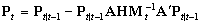
[R] xtreg, p. 437, Methods and Formulas, xtreg, re, second
paragraph
On the second line of the second paragraph of this section, make the
following change.
On the third line of the second paragraph of this section, make the following
change.
|
|
(all) |
[R] zip, p. 501, Syntax, Zero-inflated Poisson model
The option poisson should be deleted and the option
vuong inserted in the syntax diagram for zip.
|
... offset(varname) poisson probit ... |
... offset(varname) vuong probit ... |
|
|
(all) |
[R] zip, p. 501, Syntax, Zero-inflated negative binomial model
The option nbreg should be deleted and the option vuong
inserted in the syntax diagram for zinb.
|
... offset(varname) nbreg zip ... |
... offset(varname) vuong zip ... |
|
|
(all) |
[R] zip, p. 502, Options, poisson and nbreg options
The options poisson and nbreg and their descriptions
should be deleted.
|
|
(all) |
[R] zip, p. 502, Options
Add the following paragraph describing the vuong option.
|
vuong specifies that the Vuong (1989) test of the zero-inflated
Poisson model vs. the Poisson model (or zero-inflated negative binomial
model vs. negative binomial model) be reported. This test statistic has
a standard normal distribution with large positive values favoring the
zip (zinb) model and large negative values favoring the Poisson (negative
binomial) model. |
|
|
(1) |
[R] zip, p. 502, Options, zip option
The last sentence in the zip option concerning the Wald test
should be deleted.
|
zip ... The default is to include a Wald test. |
zip ... |
|
|
(all) |
[R] zip, pp. 503–504, Example
The entire example starting in the middle of p. 503 and continuing
through the middle of p. 504 has been replaced.
Click here
to view the correction.
|
|
(all) |
[R] zip, p. 507, References
Add the following entries to the References section.
|
Greene, W. H. 1994. Accounting for excess zeros and sample selection in
Poisson and negative binomial regression models. Working paper no.
EC-94-10, Department of Economics, Stern School of Business, New York
University.
Vuong, Q. 1989. Likelihood ratio tests for model section and non-nested
hypotheses. Econometrica 57: 307–334. |
Also update the Greene (1997) reference to the fourth edition.
|
Greene, W. H. 1999. Econometric Analysis, 4th ed. Upper Saddle River, NJ:
Prentice–Hall. |
|
|
(all) |
[U] 1.3.3 Changes to existing commands, p. 14, second paragraph
|
brier ... test of the ROC area being greater than .5; ... |
brier ... test that a brier score is extreme; ... |
|
|
(all) |
[U] 1.3.6 New programming features, p. 20, second paragraph under
"Other matrix changes:"
|
You can ... instead refer to A[i,...]. |
You can ... instead refer to A[i,1...]. |
|
|
(all) |
[U] 16.3.4 Time-series functions, p. 126, monthly() entry
|
monthly(s1,s2[,y)]) |
monthly(s1,s2[,y]) |
|
|
(all) |
[U] 17.9 Subscripting, p. 160, last line of item 3
|
generate hat = price*b[1,"mpg:price"] |
generate hat = price*b[1,colnumb(b,"mpg:price")] |
|
|
(all) |
[U] 21.3.5 Double quotes, p. 194, seventh line
|
Why is `"example'" better than ... |
Why is `"example"' better than ... |
|
|
(all) |
[U] 27.3.1 Inputting time variables, p. 294, sentence before the
table
|
We ... for %d variables; ... |
We ... for %t variables; ... |
|
|
(all) |
[U] 27.3.6 Creating time variables, p. 297, command after first
paragraph
|
. generate time = d(19100q1)+_n-1 |
. generate time = q(19100q1)+_n-1 |
|